Definition of the Problem and Selection of Variables:
How does time affect the position, velocity, and acceleration of the cart when rolling down a ramp?
The independent variable for this experiment was time, while the dependent variable was position.
The independent variable for this experiment was time, while the dependent variable was position.
The Controlling Variables:
The controlling variables of the experiment were the cart, the ramp, the starting position of the cart on the ramp, and the angle of the ramp. We used the same cart and same ramp for the experiment, ensuring that there would be no variation due to these variables. While we only did one trial (as the lab intended), if we had done multiple the data would not have changed due to the cart, ramp, starting position of the cart, or the angle of the ramp.
A Developed Method for the Collection of Data:
To collect sufficient and relevant data, our group used video analysis through Loggerpro. We captured a video of our cart rolling down the ramp, and put it into Loggerpro. Through video analysis, we scaled the video to mark our starting point of the cart being released as time 0. In placing a meter stick in the background, Loggerpro was able to make an accurate measurement of the position of the cart because it had a scale of reference. By then advancing the video frame by frame, we could plot our points in the graph, giving us a graph of sufficient and relevant data.
The Procedure:
The purpose of our procedure was to measure the position of the cart in respect to time when rolling down a ramp.
We initially set our camera up to capture a video of the cart going down the ramp.
We placed a meter stick in front of the ramp so that there would be a scale of reference for the video analysis.
We placed the cart at the top of the ramp, with the back wheels at the very back of the cart, holding it in place.
We then released the cart, and let it run down the ramp while the video captured it all.
We then caught the cart before it hit the table, giving us a full start to stop video of the cart going down the ramp.
Labeled Diagram: |
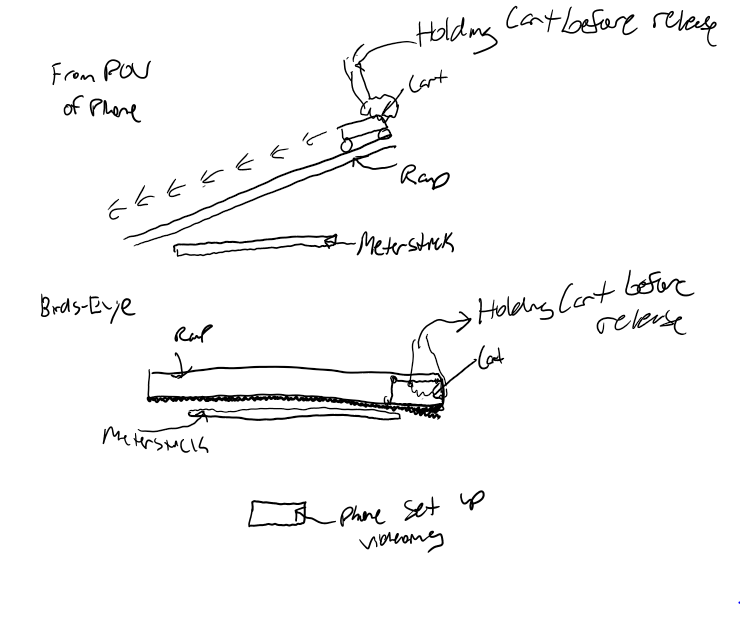
|
Processed Raw Data
The raw data was captured using video analysis. Using Loggerpro, we inserted our video, advancing frame by frame to make data points. We did not need to use any calculations, as Loggerpro created the line of best fit. The procedure largely explains how we were able to capture accurate and reliable data.
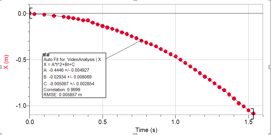
Position-Time Graph:This is the Position-Time graph of the cart going down the ramp. The x-axis represents the time in seconds, while the y-axis represents the position in meters. As we can see in the graph, our equation of best fit is a quadratic model. The slope of this graph represents the velocity of the cart on the time interval. The slope gets steeper and steeper as time goes on, showing an increase in speed as the cart goes down the ramp. The y-intercept value of -0.005087 represents the starting position of the cart. This value is approximately 0, which makes sense as the cart has moved 0 meters at 0 seconds.
The equation for the best fit of the Position-Time graph is P(t)= -0.4446t^2 + -0.02934t + -0.005087 |
|
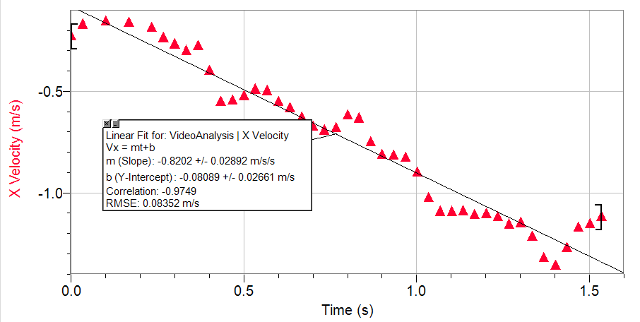
Velocity-Time Graph:This is the Velocity-Time graph of the cart going down the ramp. The x-axis represents the time in seconds, while the y-axis represents the velocity of the cart in meters per second. As we can see in the graph, our equation of best fit is a linear model. The slope of this graph represents the acceleration of the cart on the time interval. The slope is a negative constant, showing that the acceleration is a negative value and velocity is decreasing over time. The y-intercept of -0.08089 is the initial velocity of the cart, which is approximately 0. This makes sense because the cart was being held in place to start, not moving at all.
The equation for the best fit of the Velocity-Time graph is V(t)= -0.8202t + -0.08089 |
|
Conclusion:
The purpose of this lab was to evaluate the relationship between position and time. Through this relationship, we could also evaluate how the velocity and the acceleration of the cart varied over time. We could conclude after this experiment that the cart moving down the ramp in a negative direction resulted in a graph where the slope (velocity) got steeper and steeper, making the slope a larger negative number as time went on. This can be seen in both the Position-Time graph and the Velocity-Time graph. In the Position-Time graph, our line of best fit was an upside down quadratic function, whereas as time increased the position decreased at an increasing rate. The slope of the Position-Time graph was getting more and more negative as time went on, meaning that it is getting steeper. In the Velocity-Time graph, we see a linear equation as our line of best fit. This linear equation had a constant negative slope, showing how the velocity is getting to be a much larger negative number as time went on. The slope of the Velocity-Time graph gives us the acceleration, which is simply a flat line. This lab was able to help us understand how position, velocity, and acceleration were all correlated in regards to time. We can generalize that the position is determined directly by the time, the velocity is the slope of the position-time function, and the acceleration is the slope of the velocity-time function. From this, we can generalize that a quadratic position-time function will give us a linear velocity-time function which will give us a flat line acceleration-time function. This lab shows how position, velocity, and acceleration are all related and interconnected to time, and how that mathematical application is seen in real life motion.
Evaluating and Improving:
The two most significant sources of uncertainty in the lab were the graphical point collection technique and the shortness of the ramp. In gathering our points for our graph, we had to advance frame by frame and click on the front of the car. However, due to blurry imaging and an unreliable mouse pad, this measurement was not as accurate as it could have been. This might have caused a slight alteration to our data that could have largely affected our analysis, or made our data unreliable. The shortness of the ramp left no room for error, as well as little chance for observation. Because the ramp is so short, the time values are very small. This means that any slight miscalculation in data points (which is a possibility as seen above) could make the data unreliable. There is such a small range for the data that it is susceptible to small inaccuracies.
One improvement to the problem of a short ramp would be to make a longer ramp. This would create larger time values, which would make the data much more observable. More importantly, the data would be less susceptible to small inaccuracies, as they make up a much smaller proportion of the data as a whole.
One improvement to the problem of a short ramp would be to make a longer ramp. This would create larger time values, which would make the data much more observable. More importantly, the data would be less susceptible to small inaccuracies, as they make up a much smaller proportion of the data as a whole.
